Psychological Scaling using MLDS
In this tutorial, I’ll walk you through how to implement Maximum Likelihood Difference Scaling in R. See (Knoblauch & Maloney, 2012, chap. 7) for full details.
This tutorial was written in R, using RMarkdown to generate this webpage. You can access the markdown file here. I make heavy use of tidyverse (Wickham et al., 2019) throughout, so if you don’t have/use that package you’ll need to rework some of the code.
What is psychological scaling?
Psychological scaling is a technique that takes behavioral responses to stimuli that vary along some dimension and attempts to “scale” them to identify the underlying psychological structure of the stimulus space. For example, take the circular color space shown below - we have 360 different colors, each defined in terms of their “angle” around the circle. Implicitly, this structuring of the stimulus space (by us, the experimenters) suggests that the stimuli should be consistently spaced (e.g., 60° is twice as far between colors compared to 30°).

Here, we are interested in comparing distances between stimuli, such as the perceived similarity between two items on a display, or between an item held in mind and another on a display (as is common in many cognitive studies). The representation of these distances (i.e., the psychological similarity) may not map linearly onto the distances in the stimulus space, and indeed this is true for many types of stimuli (as we’ll see for color here).
What does a psychological scaling task look like?
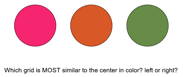
To estimate how a feature like color is scaled in psychological representations, we can get participants to perform a similarity judgement task. In these tasks, we present participants with a set of stimuli and ask them to make some judgement about the relative similarity of the items along the dimension of interest. For example, in a “triad” similarity task we can present participants with one reference stimuli and two candidate stimuli, and simply ask them which of the two candidates is most similar to the reference.

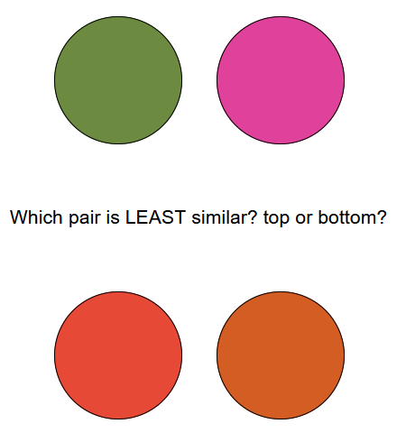
We can also present them with two pairs of stimuli (a “quad” similarity task) and ask which of the two pairs is most similar to one another.

Here, the exact colors of the items are irrelevant to the task, and we can vary them randomly from trial to trial. Importantly, both versions of this task require participants to assess the distance between the stimuli along the feature dimension we care about (e.g., color) and determine which distance is greater/smaller. In this way, their responses reveal to the experimenter something about how the distances are represented internally (i.e., the psychological scaling). But how do we take those responses and turn them into some estimate of the participant’s “scaling” function? This is where MLDS comes in.
How do we calculate the scaling function?
Once you have data, we can fit the MLDS model easily using GLM methods. Knoblauch and Maloney (2012) also describe methods for fitting through direct optimization, however the two methods will lead to very similar scaling estimates.
Before we fit the model, let’s consider how our data is structured. Here’s the first few trials from the triad task for one participant:
| trialNum | diffL | diffR | saidL | RT | trialacc | SID |
|---|---|---|---|---|---|---|
| 1 | 180 | 60 | FALSE | 3879 | 1 | 32 |
| 2 | 30 | 90 | TRUE | 2192 | 1 | 32 |
| 3 | 0 | 30 | TRUE | 956 | 1 | 32 |
| 4 | 50 | 0 | FALSE | 677 | 1 | 32 |
| 5 | 60 | 90 | TRUE | 1655 | 1 | 32 |
| 6 | 40 | 10 | FALSE | 1165 | 1 | 32 |
On each trial, we save out the difference in color angle between the reference color and the left item (diffL) and right item (diffR), as well as the participants’ choice for which color is most similar to the reference color (saidL). These are going to be the data columns we use for modelling. We could also use their accuracy on each trial; it’s mathematically equivalent, but requires recoding the left and right angles to whether they are the correct choice on a given trial (try it yourself and compare!). Here, we’re predicting the probability of the participant picking the left stimulus as most similar, rather than the probability of picking the correct stimulus.
This format is going to remain consistent when analyzing the quad task, as you can see from the structure of that data:
| trialNum | diffTop | diffBot | saidTop | RT | trialacc | SID |
|---|---|---|---|---|---|---|
| 1 | 90 | 120 | TRUE | 2299 | 1 | 9229 |
| 2 | 120 | 10 | FALSE | 1520 | 1 | 9229 |
| 3 | 30 | 90 | FALSE | 1436 | 0 | 9229 |
| 4 | 90 | 40 | FALSE | 1506 | 1 | 9229 |
| 5 | 40 | 180 | TRUE | 1362 | 1 | 9229 |
| 6 | 10 | 40 | TRUE | 2375 | 1 | 9229 |
In both cases, we ignore the identity of the individual items, and just code the angle difference between the pairs (or relative to the reference color).
Because of the similarity in how we fit the data from each task, I’ll just use the quad task data from this point on (mostly because the experiment I’m taking it from has more trials overall).
Fitting the GLM
Although the name may sound intimidating, actually fitting the Maximum Likelihood Difference Scaling (MLDS) model is pretty simple. Essentially, we are estimating the scaling parameters using logistic regression. However, we do have to go one step beyond how you would fit a normal regression model. In this case, we can’t just regress the color angle differences onto participants responses, because 1) responses are going to be a function of the relationship between the similarity of the top and bottom colors (that is, they aren’t just independent predictors), and 2) any given difference in color (say, 20° from the reference color) can be the correct choice on one trial (if the alternative is 60° from the reference) but the incorrect choice on another trial (if the alternative is only 10° different from the reference).
This means we have to fit the model slightly more directly, by first constructing the full design matrix, which we then regress onto participants’ responses. If you’ve ever taken an upper-level course in regression models or GLMs you’ve probably done this before, but even if you haven’t the idea is not too complicated. The design matrix is just a way of encoding into your model the levels of different variables in your data: in a one-way ANOVA, for example, the design matrix contains a column for each level of your independent variable, and each column records a 1 if the condition is present or a 0 if it is absent; in linear regression, each column is a continuous predictor variable with different values on each row for each observation (e.g., individuals’ heights).
For MLDS, we are going to have a column for each possible difference level, and each column will record if that difference was shown on the top (-1), on the bottom (1), or not shown (0). You can code this using other values too, but the choice of -1 and 1 is particularly convenient. We choose these values, because as the difference between the colors on the top gets larger, participants should be less likely to choose the top, while as the difference on the bottom gets larger, participants should be more likely to choose the top.
So, let’s build a design matrix! You can do this in any way that works for you, however the R code below should work with some adaptations to your particular experiment setup.
stim_diffs <- c(0,10,20,30,40,60,90,120,180) # color angle differences used

# first, generate indices for each stim diff to help fill the matrix
data_quad <- data_quad %>%
  mutate(diffTopIdx = match(diffTop, stim_diffs),
         diffBotIdx = match(diffBot, stim_diffs))

quad_mat <- matrix(0, nrow = nrow(data_quad), ncol = length(stim_diffs)) # fill matrix with 0's
colnames(quad_mat) <- paste0("stim",stim_diffs) # give the columns titles

# loop over trials and fill in the matrix
for(ii in 1:nrow(quad_mat)) {
  quad_mat[ii, data_quad$diffTopIdx[ii]] <- -1 # top diffs are -1
  quad_mat[ii, data_quad$diffBotIdx[ii]] <- 1  # bottom diffs are 1
}

quad_mat %>% head # check the first few rows for consistency
##      stim0 stim10 stim20 stim30 stim40 stim60 stim90 stim120 stim180
## [1,]     0      0      0      0      0      0     -1       1       0
## [2,]     0      1      0      0      0      0      0      -1       0
## [3,]     0      0      0     -1      0      0      1       0       0
## [4,]     0      0      0      0      1      0     -1       0       0
## [5,]     0      0      0      0     -1      0      0       0       1
## [6,]     0     -1      0      0      1      0      0       0       0
You should be able to compare this matrix to the data shown earlier. For the first trial: the color difference on top was 90°, which receives a -1 in the design matrix; the color difference on the bottom was 120°, which receives a 1 in the design matrix.
But, we’re not quite done yet. Because every row of the design matrix contains both a 1 and a -1, the sum of every row is 0. This means that our matrix is singular and the model will not fit. We solve this by discarding the first column of the matrix, corresponding to when the difference between colors on the top or bottom is zero (i.e., the pair are the same color). This does two useful things: it allows the model to be fit (always a plus), and it also fixes the output variables along our scale so that a 0° difference corresponds to a scaling value of zero (which helps interpreting the other scale values too).
quad_mat <- quad_mat[,-1] # drop the first column
Now we can fit our model. If you prefer, you can do this by constructing a data frame that combines participants’ responses with the design matrix, but I’m just going to fit things using these structures separately.
We fit the MLDS model using the base ‘glm’ function in R, but specifying a logistic regression (specifically a “probit” model) as we are predicting a binary output (participants either select the left item, or not). We also remove the intercept from the model (the ‘-1’ in the model specification below), because we are fixing the scale intercept at 0, as mentioned above.
# model specification
scaling_fit <- glm(data_quad$saidTop ~ quad_mat -1, family = binomial("probit"))
summary(scaling_fit)
##
## Call:
## glm(formula = data_quad$saidTop ~ quad_mat - 1, family = binomial("probit"))
##
## Deviance Residuals:
##     Min       1Q   Median       3Q      Max
## -3.0052  -0.0694   0.0001   0.1814   3.9579
##
## Coefficients:
##                 Estimate Std. Error z value Pr(>|z|)
## quad_matstim10    1.3573     0.5183   2.619  0.00883 **
## quad_matstim20    2.8965     0.6823   4.245 2.18e-05 ***
## quad_matstim30    3.4556     0.7079   4.882 1.05e-06 ***
## quad_matstim40    4.1567     0.7277   5.712 1.11e-08 ***
## quad_matstim60    4.8268     0.7452   6.477 9.37e-11 ***
## quad_matstim90    5.7482     0.7725   7.441 1.00e-13 ***
## quad_matstim120   6.2516     0.7882   7.932 2.16e-15 ***
## quad_matstim180   6.9761     0.8158   8.551  < 2e-16 ***
## ---
## Signif. codes:  0 '***' 0.001 '**' 0.01 '*' 0.05 '.' 0.1 ' ' 1
##
## (Dispersion parameter for binomial family taken to be 1)
##
##     Null deviance: 548.97  on 396  degrees of freedom
## Residual deviance: 122.65  on 388  degrees of freedom
## AIC: 138.65
##
## Number of Fisher Scoring iterations: 8
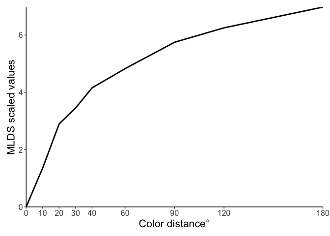
The coefficients from this model are our scaled values, so let’s quickly plot them (and also include the point at zero).

But what do these scale values actually mean? Because we used the probit link function in our model, these values are interpretable as quantiles from the cumulative normal distribution. To show you that this is true, we can calculate the probabilities ourselves!
For example, take the scale value for a color distance of 10° (1.357). Implicitly, this is the quantile for the comparison between pairs with 0° and 10° color distance. If we look at the data for trials with differences of 0° and 10°, we find that this participants’ average accuracy is 0.909. Then, if we compare with the cumulative normal distribution, we find that Φ(1.357) = 0.913. Pretty close!
We can do this for comparison between any pair of distances! The values we get out of the model are all relative to 0°, but we can take differences between values to compare those points too. Take, for example, the difference between 90° and 180°. When comparing pairs that differed by these distances, the participant in our data had an average accuracy of 0.818, and if we compared the scale values we find that Φ(6.976-5.748) = Φ(1.228) = 0.89.
The model fit is a little bit off here, predicting better performance than we actually observe, but this demonstrates the limitation of looking at comparisons like this in isolation. In this dataset, for example, there are only 11 trials for each pair of comparisons, but 36 possible comparisons between all differences. When fitting the model for each point, it’s not trying to fit perfectly to individual comparisons like we have looked at here (i.e., the “local” structure), but all comparisons that exist in the data (the “global” structure).
Holistically, the model output is consistent with what we observe in the data: participants are better at judgments between pairs that are lower overall in distance (that are more similar, e.g., 0° vs 30°) than pairs that are further in distance (e.g., 90° vs 180°).
Conclusions
I hope this helped provide an intuitive explanation of what psychological scaling is, and how you can use MLDS to estimate it. For examples of how it can be used in psychological studies more generally, you can check out the original MLDS paper (Maloney & Yang, 2003), the TCC model of working memory (Schurgin et al., 2020), or one of my own papers comparing visual search performance as a function of distance in stimulus space or psychological space (Chapman & Störmer, 2022).
Feel free to reach out to me if you have any questions, comments, or suggestions!
References
- Knoblauch, K., & Maloney, L. T. (2012). Modeling Psychophysical Data in R. Springer Science and Business Media. https://doi.org/10.1007/978-1-4614-4475-6
- Wickham, H., Averick, M., Bryan, J., Chang, W., McGowan, L. D. A., François, R., Grolemund, G., Hayes, A., Henry, L., Hester, J., Kuhn, M., Pedersen, T. L., Miller, E., Bache, S. M., Müller, K., Ooms, J., Robinson, D., Seidel, D. P., Spinu, V., … Yutani, H. (2019). Welcome to the tidyverse. Journal of Open Source Software, 4(43), 1686. https://doi.org/10.21105/joss.01686
- Maloney, L. T., & Yang, J. N. (2003). Maximum likelihood difference scaling. Journal of Vision, 3, 573–585. https://doi.org/10.1167/3.8.5
- Schurgin, M. W., Wixted, J. T., & Brady, T. F. (2020). Psychological scaling reveals a unified theory of visual memory strength. Nature Human Behavior, 4, 1156–1172. https://doi.org/10.1038/s41562-020-00938-0
- Chapman, A. F., & Störmer, V. S. (2022). Feature similarity is non-linearly related to attentional selection: evidence from visual search and sustained attention tasks. Journal of Vision, 22(8), 4. https://doi.org/10.1167/jov.22.8.4
